|
MATLAB
RESOURCES INTRODUCTION
TO QUANTUM MECHANICS
3rd
Edition
David
J Griffiths & Darrel F Schroeter
Ian
Cooper matlabvisualphysics@gmail.com CHAPTER 2 THE SCHRODINGER EQUATION THE HARMONIC OSCILLATOR HERMITE POLYNOMIALS DOWNLOAD DIRECTORY FOR MATLAB SCRIPTS QMG23C.m Griffith
in section 2.3.2 used an analytically method to solve the Schrodinger
equation which uses Hermite polynomials. Again, much mathematics and little
physics. With software such as Matlab and fast computers with lots of memory,
a better approach is to use numerical methods. I will
consider the truncated parabolic potential discussed in the previous chapter. https://d-arora.github.io/Doing-Physics-With-Matlab/mpDocs/QMG2D.htm The
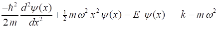
Schrodinger equation for the harmonic oscillator is The
normalized solution of the Schrodinger equation given by Griffiths is where
the scaled position is The
Script QMG23C.m can be used to investigate the analytical solution in
more detail than is given in Griffiths’ text. The
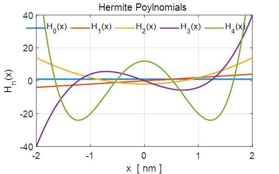
Matlab function hermiteH(n,x) is used to evaluate the Hermite polynomial. For example,
to calculate the first 5 orders and plot the results: % Hermite polynomials
=============================================
NP = 5;
Hn = zeros(NX,NP);
xH = linspace(-2,2,NX);
for c = 1:NP Hn(:,c) =
hermiteH(c-1,xH);
End
Fig.
1. The first 5 Hermite
polynomials n = 0, 1, 2, 3 and 4. The
parabolic potential energy function is defined in terms of
Position
is generally measured in nanometres (nm) and energy in electron volts (eV)
for an electron bound in the parabolic well. Results of
the simulation for the electron trapped in the parabolic well are displayed
graphically.
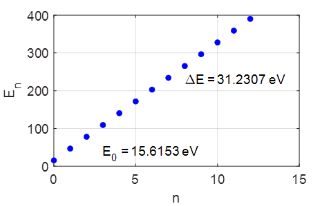
Fig.
2. The first 6 total energy
levels for the harmonic oscillator. The
quantized energy levels are given by
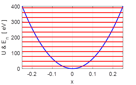
Fig.
3. The potential
energy function and the quantized energy levels. Note: the energy levels are
equally spaced, the separation between adjacent levels being
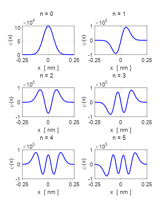
Fig.
4. The first 6 eigenfunctions or
stationary states of the harmonic oscillator. From
figure 4, it is clear that
Fig. 5.
The potential energy U, kinetic energy
K and total energy E for the
stationary state n = 2 (top) and the wavefunction (bottom).
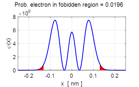
Fig.
6. The probability density
for the stationary state n = 2. The red coloured areas represent the
classically forbidden region. In the
region –0.13 < x <
0.13 (between the vertical blue lines) the kinetic is positive, outside this
region the kinetic energy is negative and is called the classical forbidden region, since a
classical particle could not move into this forbidden region where the
kinetic energy is negative. However, the probability of locating the particle
in the forbidden region is not zero as the wavefunction penetrates this classically
forbidden region. It is immediately obvious that the probabilities obtained
classically and quantum mechanically are very different. According to the
classical view of the harmonic oscillator, the probability of finding the
particle is greatest near the limits of oscillation and there is zero
probability that the particle is beyond those limits. According to quantum
mechanics, the highest probability of locating the particle is not at the
limits and may even occur at the equilibrium position and there is a small
but non-zero probability of finding the particle beyond the limits of
oscillation. For the stationary state n = 2, on making repeated
measurements on identical systems, the probability of locating the electron
in the classically forbidden area is about 2%
which is not an insignificant number.
|