|
MATLAB
RESOURCES QUANTUM
MECHANICS
Ian
Cooper matlabvisualphysics@gmail.com TIME DEPENDENT SCHRODINGER EQUATION FINITE DIFFERENCE TIME DEVELOPMENT METHOD WAVE-PACKET SPREADING DOWNLOAD DIRECTORY FOR MATLAB SCRIPTS QMG24C.m [1D] time dependent Schrodinger Equation
using the Finite Difference Time Development Method (FDTD). link WAVE-PACKET
SPREADING As an example of solving the[1D] time
dependent Schrodinger equation for a free particle, let’s consider an
initial state described by the Gaussian function where A is a
normalized constant and is calculated so that In the
Script QMC24C.m, the initial state (t = 0) of
the wave-packet is expressed in terms of its real
(yR) and imaginary (yI) parts
where the imaginary part is zero. yR = exp(-0.5.*((x-x(nx1))./s).^2; yI = zeros(1,Nx); An
animation of the time evolution of the wave-packet is shown in figure 1.
Fig.
1. Animation of the wave-packet
from its initial state. The top graph shows the real
part of the wavefunction, the middle graph the imaginary
part, and the bottom graph, the probability density. You will notice that the width of the
wave-packet grows with time, i.e., wave-packet
spreading.
Although,
the wavefunction develops real and imaginary parts, both of which have lots
of wiggles, the probability density turns out to be another Gaussian function
with a width that increases with time. Eventually, the width of the
wave-packet is proportional to time (figure 2).
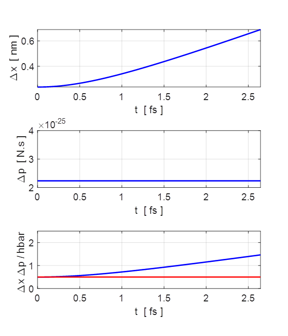
Fig.
2. The uncertainties in the
position The
initial wavefunction has a spread of momentum and this distribution of
momentum remains constant for a free particle because there are zero forces
to change it. Since there is a spread in possible momenta, there is also a
spread in velocities The
wave-packet does not propagate, it only spreads, since there are zero forces
acting on the particle. So, the expectation values of momentum, total energy,
kinetic energy and potential energy are constants, independent of time.
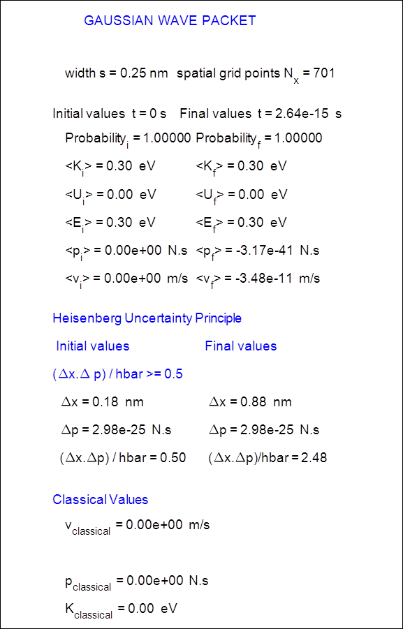
Hence, the wave-packet cannot move through space, it can only expand. Table 1.
Summary of the simulation parameters and computed results.
Note:
that increasing the spatial extent of the initial wave-packet decreases the
spread of momenta, and therefore decreases the rate at which the wave-packet
spreads (figures 3, 4 and Table 2).
Fig. 3. Animation of the wave-packet
from its initial state. The top graph shows the real
part of the wavefunction, the middle graph the imaginary
part, and the bottom graph, the probability density.
Fig. 4. The uncertainties in the position
Table 2.
After
2.64 fs s = 0.25 nm s = 0.33 nm If you
want to construct a wave-packet that remains compact for a long time, you
need to start with a very wide initial wave-packet. |