DOING PHYSICS WITH MATLAB

NEURONES AS NONLINEAR DYNAMICAL SYSTEMS

Neurone Models for [1D] Dynamical Systems

Ian Cooper

Email: matlabvisualphysics@gmail.com

MATLAB SCRIPTS

DOWNLOAD DIRECTORY

np002B.m

The function ode45 is used to solve the equation of motion to calculate the time evolution of the membrane potential for different models. To obtain the plots in this article, the Script needs to be modified by commenting and uncommenting the close all and hold on statements and by changing the plot parameters. The Script models the nonlinear dynamical system for a leak current / fast sodium ion current to simulate the upstroke of an action potential. For the leak current model, let GNa = 0 (zero sodium conductance).

np001.m

Simplified version of Script np002B.m for leak current only. Comparison of numerical and analytical solutions.

np001A.m

Simplified versions of Script np002B.m for leak current / sodium ion current with a constant sodium conductance.

np003.m

Script can be used to give the phase portrait plot and time evolution of the state variable x for systems of the form . The Script is divided into three Cells.

Cell1: Phase Portrait Plot: Define function in Cell 1

Cell 2: Time Evolution of State Variable: Solve equation of motion

Cell 3: Define function in Cell 3 at end of Script

Different functions can be modelled by changing the Script in Cells 1 and 3.

Includes code for finding the zero of a function.

np003A.m

An extension of Script np003.m for systems of the form . The Script is used to model saddle-node bifurcations for different values of the bifurcation parameters b.

INTRODUCTION

This document is based upon the book by Eugene M. Izhikevich

Dynamical Systems in Neuroscience: The Geometry of Excitability and Bursting

This book is devoted to a systematic study of the relationship between electrophysiology, bifurcations, and computational properties of neurones. Information processing depends not only on the electrophysiological properties of neurones but also on their dynamical properties. 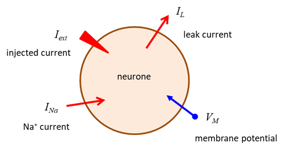Even if two neurones in the same region of the nervous system possess similar electrophysiological features, they may respond to the same synaptic input in very different manners because of each cell’s bifurcation dynamics.

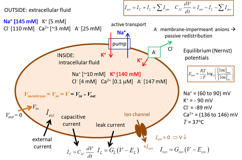
Electrical activity in neurones is sustained and propagated by ion currents through neurone membranes as shown in figure 1. Most of these transmembrane currents involve four ionic species: sodium Na⁺, potassium K⁺, calcium Ca²⁺ and chloride (Cl^-). The concentrations of these ions are different on the inside and outside of a cell. This creates the electrochemical gradients which are the major driving forces of neural activity. The extracellular medium has high concentration of Na⁺ and Cl^- and a relatively high concentration of Ca²⁺. The intracellular medium has high concentration of K⁺ and negatively charged large molecules A^-. The cell membrane has large protein molecules forming ion channels through which ions (but not A^-) can flow according to their electrochemical gradients.

The concentration asymmetry is maintained through

· Passive redistribution: The impermeable anions A^- attract more K⁺ into the cell and repel more Cl^- out of the cell.

· Active transport: Ions are pumped in and out of the cell by ionic pumps. For example, the Na⁺/K⁺ pump, which pumps out three Na⁺ ions for every two K⁺ ions pumped.

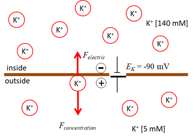
Fig. 1. Electrophysiology of a neurone.

Nernst or Equilibrium Potential

There are two forces that drive each ion species through the membrane channel.

(1) Concentration gradient: ions diffuse down the concentration gradient. For example, the K⁺ ions diffuse out of the cell because K⁺ concentration inside is higher than outside.

(2) Electric potential gradient: as ions diffuse across the membrane a charge imbalance occurs producing a potential difference between the inside and outside of the cell. For the K⁺ ions exiting the cell, they carry positive charge with them and leave a net negative charge inside the cell (consisting mostly of impermeable anions A^-), thereby producing the outward K⁺ current.

The positive and negative charges accumulate on the opposite sides of the membrane

surface creating an electric potential gradient across the membrane. This potential difference is called the transmembrane potential or membrane voltage

(1)

where the extracellular potential is the reference potential such that .

This potential slows down the diffusion of K⁺, since K⁺ ions are attracted to the negatively charged interior and repelled from the positively charged exterior of the membrane. At some point, an equilibrium is achieved. When the concentration gradient and the electric potential gradient exert equal and opposite forces on the ions, the net cross-membrane current is zero.

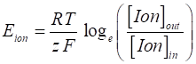
The value of such an equilibrium potential depends on the ionic species and it is given by the Nernst equation

(2)

where [Ion]_in and [Ion]_out are concentrations of the ions inside and outside the cell respectively, R is the universal gas constant (R = 8.3155 J.mol^-1.K^-1), T is temperature in degrees Kelvin, F is Faraday’s (F = (96 485 C.mol^-1), z is the valence of the ion (z = 1 for Na⁺ and K⁺, z = -1 for Cl^-, and z = 2 for Ca²⁺). E_ion is also called the reversal potential.

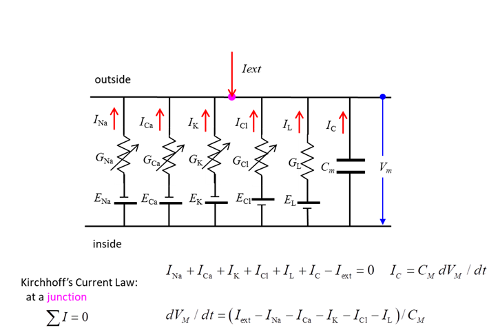
Fig. 2. Diffusion of K⁺ ions down the concentration creates an increasing electric force directed in the direction opposite to the force due to the concentration difference until the diffusion and electrical forces balance each other.

Membrane Currents

We can model the movement of ions across the membrane as an electric circuit as shown in figure 3.

Fig. 3. Equivalent circuit representation of a nerve cell membrane.

In the neuroscience literature, there is often some confusion and inconsistencies in the use of scientific language and the units used for physical quantities. For example, the terms conductance and conductance per unit area are often not distinguished and g maybe the conductance or conductance per unit area with units S or S.cm^-2. In Izhikevich’s book, he gives the current in A.cm^-2, which is clearly wrong.

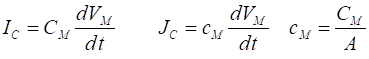
In the Scripts to model the dynamic behaviour of neurones, S.I. units are used for all input parameters and calculations. However, results may be expressed in non S.I. units, for example, mV for voltage.

The current through a resistive element can be expressed by the equation

(3)

I current [ampere A]

V potential difference [volts V]

R resistance [ohm ]

G conductance [siemens S 1 S ]

This equation can also can also be expressed in expressed in terms of the current density

(4)

A area [m]

J current density [A.m^-2]

g specific conductance [S.m^-2]

The major ion currents shown in figure 2, can be expressed as

(5)

X ion (e.g. Na⁺ K⁺ leakage)

V_M membrane potential (voltage) [volt V]

E_X equilibrium (Nernst) potential [V]

When the conductance is constant, the current is said to be ohmic. In general, ionic currents in neurones are not ohmic, since the conductance may depend upon time, membrane potential, and pharmacological agents (e.g. neurotransmitters). It is the time-dependent variation of conductances that allow a neurone to generate an action potential (spike).

The membrane acts like a capacitor – an insulator (membrane) surrounded by the extracellular and intracellular fluids (conductive plates). When the membrane potential changes, a current is generated to charge or discharge the capacitor. The capacitor current is given by the time derivative of the voltage

(6)

C_M capacitance [F]

c_M specific capacitance [F.m^-2]

The equivalent circuit to represent the electrical properties of membranes is shown in figure 3. According to Kirchhoff’s Current Law, the sum of the currents entering and leaving a junction must add to zero. Hence across the membrane

(7)

Therefore, we can write an “equation of motion” to describe the dynamical system of a neurone as

(8)

Note: are inward currents (outside to inside)

are outward currents (inside to outside)

The membrane potential is typically bounded by the equilibrium potentials

One example of the application of equation (8) is the Hodgkin-Huxley Model.

For different models of a neurone, equation (8) can be solved using the Matlab ordinary differential equation solver ode45.

GEOMETRICAL METHODS OF ANALYSIS OF [1D] DYNAMICAL SYSTEMS

In this section will start our study of the geometrical methods of analysis of [1D] dynamical systems, that is, systems having only one variable. This section is linked to Chapter 3 of Izhikevich’s book. However, the results given in this chapter using Izhikevich’s input data could not be reproduced using my Scripts. I had to change the numerical values used for the simulations.

In general, [1D] dynamical systems are described by ordinary differential equations of the form

where V is a scalar time-dependent variable which represents the state of the system. V is called a state variable.

Since , at every point V where F(V ) is negative, the derivative is negative, and hence the state variable V decreases. In contrast, at every point where is F(V ) positive, is positive, and the state variable V increases such that the greater the value of F(V ), the faster V increases. Thus, the direction of movement of the state variable V, and hence the evolution of the dynamical system, is determined by the sign of the function F(V ).

Space-clamped membrane having only a ohmic leak current

A space-claimed membrane is one in which the membrane potential is fixed by an experimenter and an external current exerted into the neurone. The space-clamped condition is so the injected current equals the net current generated by the transmembrane conductances.

Possibly, the simplest [1D] dynamical system we can look at is a neurone which has only an ohmic leak current. The equation of motion to be solved is

(9A)

(9B)

(9C)

The membrane potential V_M is the single time-dependent variable. The membrane capacitance C_M, the leak conductance G_L, and the leak reversal potential E_L are all constants.

The explicit analytical solution of equation 9C is

(9D)

where the initial value of the membrane potential is .

Equation 9C is solved numerically and analytically using the Script np001.m. using the input parameters:

% conductance [19e-3 S]

G = 19e-3;

% Membrane capacitance [10e-6 F]

C = 10e-6;

% Reversal potential / Nernst potential [EL = -67e-3 V)

E = -67e-3;

% Simulation time [5]

N = 10;

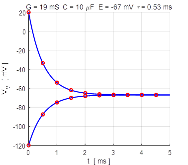
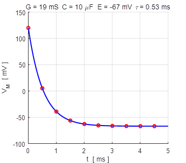
% Initial membrane voltage [0 V]

V0 = 20e-3;

The equation of motion, equation 9C is solved using the ode45 function

The Script can be run for different initial values of the membrane potential V_o and one can compare the numerical and analytical solutions as shown in figures 4A and 4B.

Fig. 4A. The membrane potential as a function of time for two different initial values of the membrane potential. The red dots show the analytical solution and the blue curve, the numerical solution. np001.m

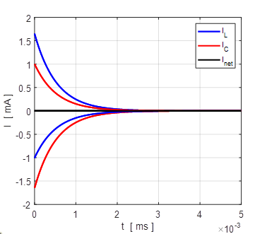
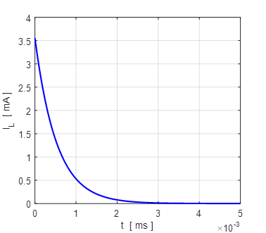
Fig. 4B. The membrane currents as function of time for two different initial values of the membrane potential. np001.m

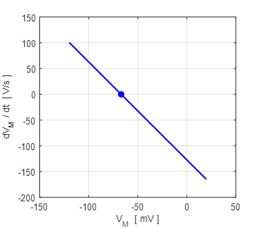
A phase portrait is a geometric representation of the trajectories of a dynamical system in the phase plane. Each set of initial conditions is represented by a different curve, or point. Phase portraits are an invaluable tool in studying dynamical systems. The phase portrait for our neurone model is a plot of the time derivative of the potential against the potential (figure 5) is a straight line. For all initial conditions, the membrane potential will be pulled to the reversal potential .

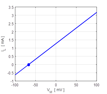
Fig. 5A. The straight line corresponds to the phase portrait plot for an ohmic element. The blue dot shows the reversal potential when time derivative of the potential becomes zero. np001.m

Also, a useful plot is the I-V characteristic curve as shown in figure 5B.

Fig. 5B. I-V characteristic curve for two different initial conditions (-100 mV and +100 mV). The blue dot represents the equilibrium point (stable equilibrium) where the final current is zero and the membrane potential equals the leak reversal potential. A positive value of the current indicates an outward current to decrease the membrane potential while a negative current is an inward current which increases the membrane potential. The straight means that the conductance is constant and the slope of the line gives the numerical value of the conductance (G = 19 mS).

In our simple model, the steady-state solution of the equation of motion 9C is

(10)

The point is a point of stability (stable equilibrium). For all initial values of the membrane potential, the system will evolve such that .

Fig.6. The initial membrane voltage is reduced to the leak reversal potential (steady-state) by a net outward current (net movement of positive charge from inside to outside the cell membrane) that hyperpolarizes the membrane. If the initial value of the membrane potential was less than the reversal potential, then a net inward current would depolarize the membrane.

In the qualitative analysis of any dynamical system it is important to find the equilibria or rest points, i.e., the values of the state variable where F(V) = 0 and V is an equilibrium value. At each such point , the state variable V does not change. In the context of membrane potential dynamics, equilibria correspond to the points in the phase portrait plot where . At each such point there is a balance of the inward and outward currents so that the net transmembrane current is zero, and the membrane voltage does not change. For our ohmic leak current model, there is only one equilibrium point since the phase portrait plot (figure 5) is a monotonic decreasing function.

We can add to our model a sodium ion channel which has a constant conductance. The equation of motion for our model is

(11)

Equation (11) is solved using the Script np001A.m with input parameters

% conductance [19e-3 74e-3 S]

GL = 19e-3; GNa = 74e-3;

% Membrane capacitance [10e-6]

C = 10e-6;

% Reverse potential / Nernst potential [EL = -67e-3 V ENa = 60e-3)

EL = -67e-3; ENa = 60e-3;

% Simulation time [13-3 s]

tMax = 1e-3;

The results are displayed in figures 7, 8 and 9.

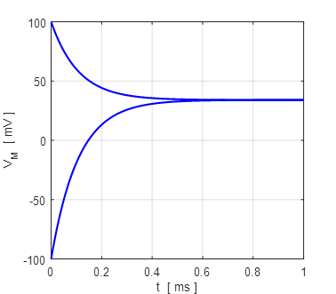
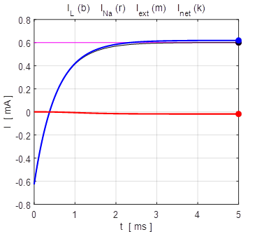
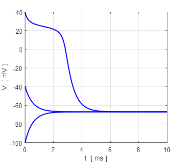
Fig. 7. The membrane potential V_M evolves to its equilibrium value of +34 mV from an initial value of +100 mV and -100 mV. np001A.m

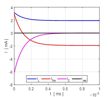
Fig. 8. The time evolution of the membrane currents. At equilibrium, the outward leakage current is balanced by the inward Na⁺ current. Initial membrane potential is +100 mV. np001A.m

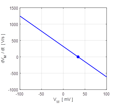
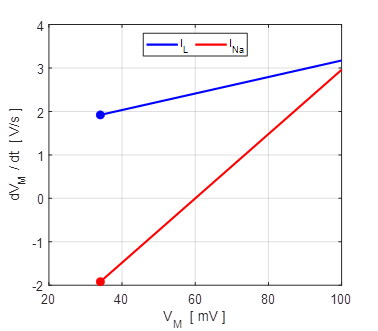
Fig. 9A. Phase portrait plot. The stable equilibrium point is (34, 0). np001A.m

The I-V characteristic plot is shown in figure 9B for the leak and sodium ion currents.

Fig. 9B. I-V characteristic plot for the leak current (blue) and sodium current (red). When a steady-state is reached (shown by the two dots), the outward flow of the leak current is balanced by the inflow of sodium ions.

Space-clamped membrane having only a ohmic leak current and sodium ion channel: Leak / fast Na⁺ model

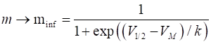
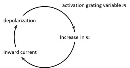
We can extend our simple model further my including a voltage dependent sodium ion channel and not an ohmic Na⁺ channel. The conductance of an ion channel is time and voltage sensitive. We will consider a space-clamped membrane having a leak current and a fast voltage-gated sodium ion current having only one variable m. The gating process is assumed to be instantaneous such that the variable m is equal to its asymptotic value m_inf where

(11)

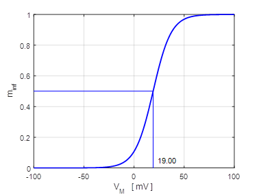
Fig. 10. The activation function for a voltage-gated Na⁺ channel. The shape of the curve is a sigmoid function. This is an activation channel, as the channel opens when activated: conductance of membrane increases with increasing membrane potential. Constants: V_1/2 = 19 mV and k = 9.0 mV. np002B.m

The dynamics of the system is described by the equation

(12)

The Script np002B.m can be used to solve equation 12 using the ode45 function. Model parameters can be changed in the input section of the Script. Typical values are:

% INPUTS >>>>>>>>>>>>>>>>>>>>>>>>>>>>>>>>>>>>>>>>>>>>>>>>>>>>>>>>>>>>>>

% conductance [19e-3 74e-3 S]

gL = 19e-3; gNa = 74e-3;

% Membrane capacitance [10e-6]

C = 10e-6;

% Reverse potential / Nerest potential [EL = -67e-3 V ENa = 60e-3]

EL = -67e-3; ENa = 60e-3;

% Simulation time [5e-3 s]

tMax = 10e-3;

% Initial membrane voltage [0 V] unstable equilibrium 6.672903e-3

V0 = 6.5672903e-3;

% V1/2 [V] k [V]

Vh = 19e-3; k = 9e-3;

% External current input [A]

Iext = 0.60e-3;

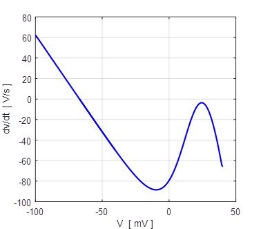
For certain input parameters, there is a “negative conductance” and our model can show a few interesting nonlinear phenomena, such as bistability (co-existence of the resting state and excited state).

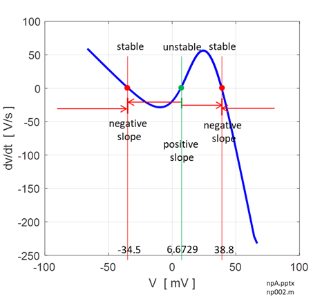
The phase portrait plot for the solution to equation 12 for different initial conditions is shown in figure 11 which shows three distinct equilibrium points where . Also, figure 12 shows the three equilibrium points. Phase portrait plots like figure 11 are important in the analysis of any dynamical system. It depicts all stable and unstable equilibria, trajectories and corresponding attraction domains in the system. It shows all possible evolutions of the state variable and how they depend upon the initial state. Looking at the phase portrait, one immediately gets all the important qualitative information about the behaviour of the system without even knowing the equation.

Fig. 11. There are two attraction domains which are separated by the unstable equilibrium point at +6.6729 mV. For any initial membrane potential, the membrane potential will converge to one of the two stable equilibrium points:  ‑ 34.5 mV (rest state) or + 38.8 mV (excited state). The red arrows show the attraction domains. An attraction domain of an attractor is the set of all initial conditions that lead to the attractor. np002B.m

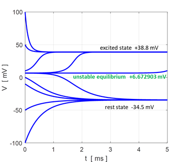
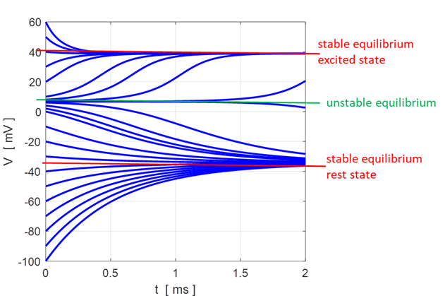
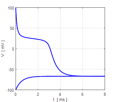
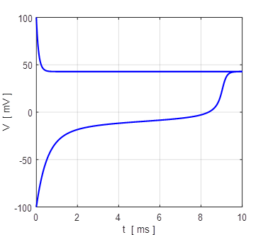
Fig. 12. Voltage trajectories for the leak / fast sodium ion model for different initial conditions. For all initial values of the membrane potential greater than the unstable membrane potential, the membrane potential is attracted to the excited state and for initial values less than the unstable equilibrium potential, the membrane potential is drawn to the resting state (bistability). The attraction to a stable equilibrium point can take a relative long time when an initial membrane potential is close to the unstable equilibrium potential. I_ext = 0.60 mA np002B.m

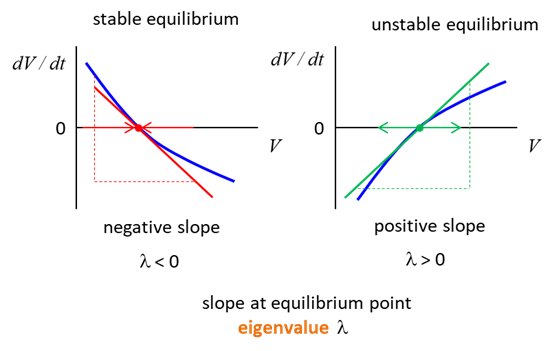
If the initial value of the membrane potential variable is exactly at equilibrium, then and the membrane potential will stay there forever.

If the initial value is near equilibrium, then the membrane potential may approach or diverge from it. At an equilibrium point, when the slope of the curve is negative, then the equilibrium is stable. We say that an equilibrium is asymptotically stable if all solutions starting sufficiently near the equilibrium will approach it as . Hence, a stable equilibrium point attracts all nearby solutions, and is called an attractor. In a [1D] system, an attractor is the only type of stable equilibrium.

At an equilibrium point, when the slope of the curve is positive, then the equilibrium is unstable. All solutions starting sufficiently near the equilibrium will diverge from it as . Hence, an unstable equilibrium point repels all nearby solutions, and is called a repeller. If a [1D] system has two stable equilibrium points, then they must be separated by at least one unstable point (figure 11) since the slope of a stable equilibrium point is negative. At membrane potentials near an unstable point, the membrane potential can diverge either to the rest state or excited state depending on whether the membrane potential is slightly lower or greater than the unstable value. Unstable equilibria play the role of thresholds in [1D] bistable systems (systems having two attractors). Suppose the membrane potential is just below the unstable value when a perturbation increases the membrane potential. If the perturbation is small and sub-threshold, the membrane potential will be attracted to the resting state. However, a larger perturbation may increase the membrane potential about the unstable value and the membrane potential will be attracted to the excited state. This perturbation is called super-threshold or supra-threshold. Thus, the unstable equilibrium acts as a threshold that separates two states.

Fig. 12A. The slope of the curve at an equilibrium point is called the eigenvalue and the sign of the slope determines the stability of the equilibrium.

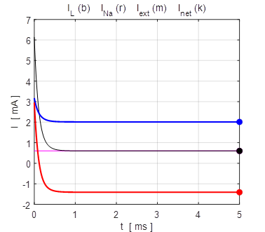
The slope of the curve at an equilibrium point is called the eigenvalue and the sign of the slope determines the stability of the equilibrium (figure 12A). Eigenvalues play an important role in determining the types of equilibria of multi-dimensional systems.

Figure 13 shows the time evolution of the leak current I_L, Na⁺ current I_Na the external current I_ext, and the combined current I_L + I_Na. The upper plot is for V0 = + 100 mV and the lower plot V0 = - 100 mV. At an equilibrium point the net current or combined current is equal to the external current . When , then the outward current balanced the inward current so that the net transmembrane current is zero.

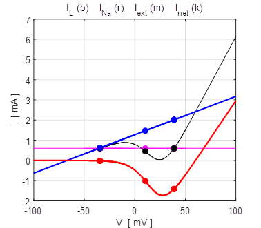
Fig. 13. The time evolution of the membrane currents: leak current I_L, Na⁺ current I_Na the external current I_ext, and the combined current I_L + I_Na . The upper plot is for V0 = + 100 mV (stable equilibrium + 38.8 mV) and the lower plot V0 = - 100 mV (stable equilibrium + 38.8 mV). np002.m

Figure 14 shows the I-V characteristic plot: leak current I_L, Na⁺ current I_Na, the external current I_ext, and the combined current I_L + I_Na. The shape I-V characteristic curve for the combined current I_L + I_Na agrees very well with measured data from layer 5 pyramidal cells in a rat visual cortex. The slope of the I-V curve is equal to the conductance. For a region of membrane potentials, the slope has negative values and hence “negative conductance”. This negative conductance creates a positive feedback between the voltage V_M and the gating variable m_inf (figure 10), and it plays an amplifying role in neurone dynamics. Such currents are referred to as amplifying currents.

Fig. 14. The I-V characteristic plot: leak current I_L, Na⁺ current I_Na the external current I_ext, and the combined current I_L + I_Na np002.m

When the external current is set to zero, I_ext = 0 A, there is only one stable equilibrium point, and the trajectory of the membrane potential is pulled a resting state.

Fig. 15. All trajectories for different initial membrane potentials are attracted to the single stable equilibrium point, V_M = - 67 mV (monostability).

Fig. 16. There is only one point where at V_M = - 67 mV. This is the single stable equilibrium point (monostability).

The transition between two stable states separated by a threshold is relevant to the mechanism of excitability and generation of action potentials of many neurones. In our Leak / fast Na⁺ model, the existence of the rest state is largely due to the leak current I_L, while the existence of the excited state is largely due to the persistent inward Na⁺ current I_Na. Small (sub-threshold) perturbations leave the state variable in the attraction domain of the rest state, while large (super-threshold) perturbations initiate the regenerative process where the upstroke of an action potential, and the voltage variable becomes attracted to the excited state.

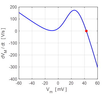
Fig. 17. Upstroke dynamics for the generation of action potential for our Leak / fast Na⁺ model. The model describes quite well the upstroke dynamics of layer 5 pyramidal neurones. I_ext = 0.60 mA np002B.m

Generation of the action potential must be completed via repolarization that moves V_M back to the rest state. Typically, repolarization occurs because of a relatively slow inactivation of Na⁺ current and/or slow activation of an outward K⁺ current, which are not taken into account our model.

BIFURCATIONS

A system is said to undergo a bifurcation when its qualitative behaviour changes. We can investigate changing the external current injected into a neurone using our leak / fast Na⁺ model.

When the external current is zero, all trajectories for initial membrane potentials are attracted to the rest state where V_M = - 67 mV (figure 18).

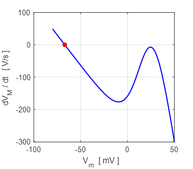
Fig. 18. I_ext = 0 mV There is only a single stable equilibrium point at the rest membrane potential V_M = - 67 mV. Monostable np002B.m

When the external current is increased Iext = 0.1 mA, then the system is bistable with stable equilibrium at -62 mV (rest state) and + 29 mV (excited state) as shown in figure 19.

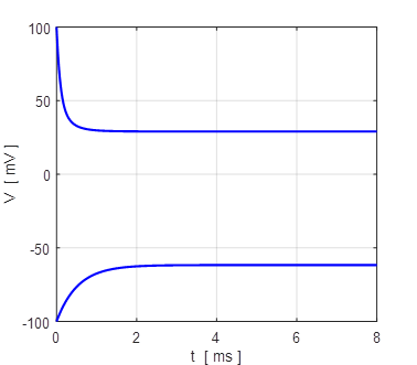
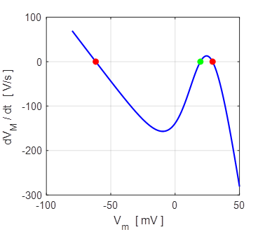
Fig. 19. I_ext = 0.1 mA There are two stable equilibrium points: rest membrane potential -62 mV and the excited state +29 mV. The unstable equilibrium point is around +20 mV. Bistable np002B.m

When the external current is greater than about 0.9 mA, there is again only one stable equilibrium point as shown in figure 20.

Fig. 20 I_ext = 0.9 mV There is only a single stable equilibrium point at the excited state membrane potential V_M = 43 mV. Monostable np002B.m

We can clearly see that the qualitative behaviour of our model depends upon the value of the external current.

I_ext = 0 mA, the system evolves to the resting state.

~0.1 mA < I_ext  <  ~0.9 mA, the system is bistable where the rest and excited states coexist.

I_ext > ~ 0.9 mA, the rest state no longer exists because the leak current cannot cope with the large injected DC injected current and the inward Na⁺ current.

When I_ext ~ 0.9 mA a saddle-mode bifurcation exists since slight variations in I_ex results in the system evolving to a bistable or monstable state. As I_ext is increased, the plot is lifted up, and the stable and unstable equilibrium approach each other. At the saddle point, they coalesce when the slope of the tangent to the curve becomes zero, and then disappear.

EXAMPLES

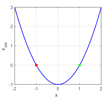
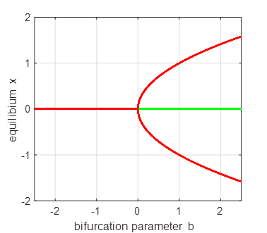
The examples given are based upon the Exercises in Chapter 3 of the Izhikevich’s book.

1. Script np003.m

System:

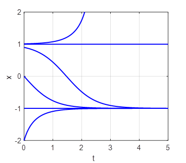
The red dot shows a stable equilibrium point and a green dot an unstable equilibrium point. For all initial values x < 1, the trajectory of the system will evolve to the stable equilibrium point at x = -1. For all values of x > 1, the trajectory of the system will diverge to infinity. The attraction domain corresponds to all initial values x < 1. The eigenvalues are the roots of the function

stable equilibrium unstable equilibrium

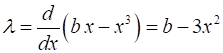
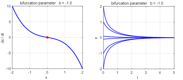
2. Script np003A.m

System: bifurcation parameter b
The dynamics of the system gives rise to a pitchfork bifurcation (saddle-node bifurcation) where b is a bifurcation parameter. Equilibria occurs when .

The eigenvalues are

If then the equilibrium is called hyperbolic and if then called non-hyperbolic.

If then there is only one solution , hence there is only one branch of equilibria. The eigenvalue is , so the equilibrium is stable.

If then there are three equilibrium points:

stable

unstable

stable

Saddle-node (fold) bifurcation diagram np003A.m

The branch losses stability when b passes the pitchfork bifurcation value of at which point a new pair of stable branches bifurcate, that is, the stable branch divides (bifurcates) into two stable branches when b passes 0.

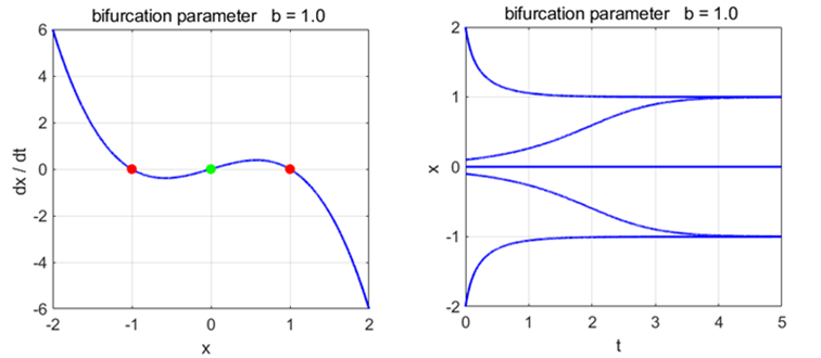
Phase Portrait and Time Evolution Plots: b = +1, 0, and -1 np003A.m