|
LORENZ
EQUATIONS Animation:
Lorenz Attractor Ian Cooper matlabvisualphysics@gmail.com DOWNLOAD DIRECTORIES FOR PYTHON CODE ds2700G.py ds2700.py Full documentation Chaos is everywhere. It can crop up in unexpected places and in
remarkably simple systems, and a great deal of work has been done to describe
the behaviour of chaotic systems. One primary characteristic of chaos is that
small changes in initial conditions result in large changes over time in the
solution curves. We can illustrate the chaotic behaviour of the Lorenz system
by animating the [3D] trajectory in phase space. To produce the animation in Python you need to: · Include
the necessary libraries - matplotlib.pyplot,
mpl_toolkits.mplot3d, and matplotlib.animation. · Solve the
Lorenz equations are integrated using the function odeint to
return the solution x(t), y(t), and z(t). · Specify
the model parameters, time span and initial conditions. · Set up
the 3D plot: Create a figure and an Axes3D object. · Initialize
the plot: Create an empty 3D line object that will be updated in each
animation frame. · Animation
function: Define a function that takes the frame number as an argument and
updates the data of the 3D line object with the calculated trajectory points
up to that frame. · Create
the animation: Use matplotlib.animation.FuncAnimation
to link the plot, the animation function, and the data, specifying the number
of frames and any other relevant parameters (like interval between frames). · Save it
as a video file MP4 or an animated gif (e.g., MP4 or GIF) using anim.save(). Figures 1 and 2 show an animation of the chaotic trajectories from two
initial conditions which are very close to each other (figure 1) and
separated (figure 2).
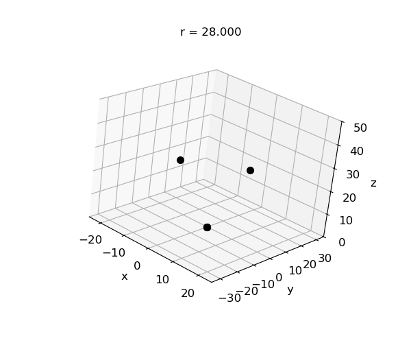
Fig. 1. Chaotic region, r
= 28. Animation of two trajectories with slightly different initial
conditions (0.10, 0, 0) and (1.15, 0, 0). For a long time at the start of the
flow, the two trajectories are almost identical. Fig. 2. Chaotic region, r = 28. Animation
of two trajectories The trajectories have a wing (lobes) around each of the non-zero fixed
points with an incoming [1D] stable direction, and two unstable manifolds
(one positive and two negative eigenvalues). The unstable manifolds are only
slightly unstable, which is why a trajectory spends a long-time winding
around a fixed point before it escapes. Note the repulsion from the unstable
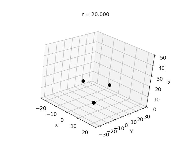
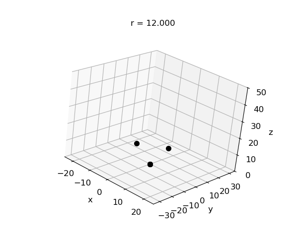
fixed point at the Origin. Figures 3 show the trajectories in the transient chaotic region and
figure 4 where the trajectories spiralling inwards to the stable fixed
points.
Fig. 3. The two
trajectories in the transient chaotic region. Both trjectroies
Fig. 4. The two
trajectories in the transient chaotic region. Both trajectories spiral
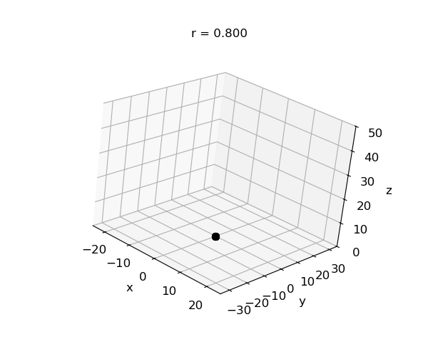
inwards to the stable fixed points. When r < 1 then the only fixed point is the Origin and all
trajectories are attracted to the stable fixed point at the Origin.
Fig. 5. r < 1,
the Origin is the only fixed point and is stable. All trajectories will be
attracted to the Origin. Animating the Lorenz System in 3D https://jakevdp.github.io/blog/2013/02/16/animating-the-lorentz-system-in-3d/ |