|
FOURIER TRANSFORM FREQUENCY SPECTRUM OF LIGHT Ian Cooper Please email
me any corrections, comments, suggestions or additions: matlabvisualphysics@gmail.com DOWNLOAD DIRECTORIES FOR PYTHON CODE
emFT01.py Individual plane
waves have infinite length and infinite duration. They do not exist in
isolation except in our imagination. Moreover, a waveform constructed from a discrete
sum (superposition
of plane waves) must be periodic as it eventually repeats over and over.
To create a waveform that does not repeat such as a single laser, we must
replace a discrete sum with an integral that combines a continuum of plane
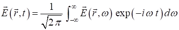
waves. Such a waveform at a point (1)
The function gives the amplitude and phase of each plane wave that
makes up the overall waveform. The operation described in equation 1 is
called an inverse Fourier transform. Given a waveform
(2)
The Fourier transform (equation 2) is used to generate
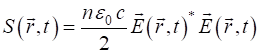
the spectrum The intensity
for continuous superpositions of plane waves is
(3)
Equation 3 specifically requires the fields to be in
complex format, and it takes care of the time-average over rapid oscillations
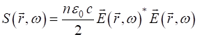
automatically. Also, equation 3 assumes that all relevant The power spectrum produced from
(4)
The power spectrum a spectral analyser or spectrometer. The total power in a signal is the
same whether we compute it in the time domain or in the frequency domain.
This result is called Parseval’s theorem.
(5)
Example Consider the waveform given by a
Gausssian function
(6)
Find the field A range of
frequencies are needed to construct a waveform that turns on and off. The
shorter the duration of the waveform, the wider the frequency spectrum that
is necessary. Note that the temporal width of the waveform is dictated by s while the
spectral width is given by Calculate the power spectrum and
check Parseval’s theorem. Python solution Usually, the
Fourier transforms are calculated by the fast Fourier transform method. In
Python and Matlab there are functions that can be implemented to find the
Fourier transforms. However, they are not easy to use as the sampling rate
and frequency domain are not independent. Historically, the fast Fourier
transform is used because of the speed of the calculations is much faster
than the direct evaluation of the Fourier integrals. But, with the speed and memory
of modern computers and using software such as Python or Matlab, the
computation of the Fourier integrals can be by the direct integration without
any problems, thus, making Fourier Transforms simple integration problem At some
arbitrary poimt, we can express the electric field for microwave frequencies (f0 = 1 GHz) as
Et = E0*exp(-t**2/(2*s**2)) * exp(-1j*w0*t) for input values nT
= 999; nF = 999
f0 = 1e9; w0 = 2*pi*f0; T0 = 1/f0
t1 = -10*T0; t2 = 10*T0
f1 = 0*f0; f2 = 1.5*f0 E0 = 1 s = 4*T0 t = linspace(t1,t2,nT) f = linspace(f1,f2,nF) w
= 2*pi*f The intensity of the wave in the
time domain SE = real(Et)**2
intensity SEE =
real(conj(Et)*Et) time-averaged
intensity In the frequency
domain #
Fourier Transform H = zeros(nF) + 1j*zeros(nF) for q in range(nF): h = Et * exp(1j*w[q]*t) HR = simps(real(h),t) HI = simps(imag(h),t) H[q] = HR + 1j*HI Ef = H/np.sqrt(2*pi) Sf = real(conj(Ef)*Ef) S = Sf/max(Sf) # Power Pt = simps(SEE,t) Pf = simps(Sf,w) Graphical output for s = 4*T0 and s = 2*T0
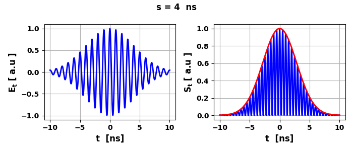
Fig.1. Time domain:
electric field and intensity of fields.
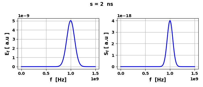
Fig.2. Frequency
domain: electric field and intensity of fields.
Pt = 7.087 nW Pf
= 7.087 nW
Fig.3. Time domain:
electric field and intensity of fields.
Fig.4. Frequency
domain: electric field and intensity of fields.
Pt = 3.545 nW Pf
= 3.545 nW Note: The narrower the electric field pulse than the wider the power
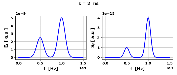
spectrum. We can add another frequency component to the electric field with
frequency 5.0 GHz Et =
E0*exp(-t**2/(2*s**2)) * exp(-1j*w0*t) Et = Et
+ (E0/2)*exp(-t**2/(2*s**2)) * exp(-1j*w0*t/2)
Fig.3. Time domain:
electric field and intensity of fields.
Fig.4. Frequency
domain: electric field and intensity of fields.
Pt = 4.431 nW Pf
= 4.431 nW The power spectrum shows the peaks at 5 GHz and 10 GHz as expected. |