|
MATLAB
RESOURCES QUANTUM
MECHANICS
Ian
Cooper matlabvisualphysics@gmail.com TIME DEPENDENT SCHRODINGER EQUATION FINITE DIFFERENCE TIME DEVELOPMENT METHOD FREE PARTICLE: GAUSSIAN WAVEPACKET PROPAGATION DOWNLOAD DIRECTORY
FOR MATLAB SCRIPTS simpson1d.m Function for [1D] integration QMG24D.m Propagation of Gaussian wavepacket ColorColde.m A
function used to represent the complex phase of the Gaussian wavepacket as a
coloured sequence. LINKS [1D] time dependent Schrodinger Equation
using the Finite Difference Time Development Method (FDTD). link Expectation values link GAUSSIAN PULSE
PROPAGATION As an example of solving the[1D] time dependent
Schrodinger equation for a free particle (unbound particle), let’s
consider an electron confined to the X axis in the region from where A is a
normalized constant and is calculated so that This
unbound state is in a classically allowed region and so the energies of the
system are not quantized and the total energy E can
vary continuously. In the
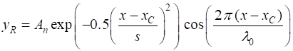
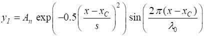
Script QMC24C.m, the initial state (t = 0) of
the wavepacket is expressed in terms of its real
(yR) and imaginary (yI) parts:
yR = exp(-0.5.*((x-x(nx1))./s).^2).*cos((2*pi).*(x-x(nx1))./wL); yI
= exp(-0.5.*((x-x(nx1))./s).^2).*sin((2*pi).*(x-x(nx1))./wL); The particle represented
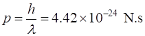
by a wavepacket is localized in space with an approximately well-defined
momentum
When the wave
packet strikes a boundary at x = 0 or x = L, reflections occur. This may cause
problems, so it may be necessary to terminate a simulation before any
reflections occur. The accuracy of the FDTD
method is improved as Simulation
parameters for Script QMC24D.m Nx
= 701
number of grid points for x-axis Nt =
7000
number of time steps L = 5x10⁻⁹
m
simulation region xC = 1x10⁻¹⁰
m
centre of pulse S =
L/25
width of pulse
An
animation of the time evolution of the Gaussian wavepacket is shown in figure
1.
Fig.
1. Animation of the
Gaussian wavepacket from its initial state. The top graph shows the real part of the wavefunction, the middle graph
the imaginary part, and the bottom
graph, the probability density.
Fig.
2. The uncertainties in the
position You will notice that the width of the
wavepacket grows with time, i.e., wavepacket
spreading.
Although,
the wavefunction develops real and imaginary parts, both of which have lots
of wiggles, the probability density turns out to be another Gaussian function
with a width that increases with time. Eventually, the width of the
wavepacket is proportional to time (figure 2). The
initial wavefunction has a spread of momentum and this distribution of
momentum remains constant for a free particle because there are zero forces
to change it. Since there is a spread in possible momenta, there is also a
spread in velocities The
wavepacket as it spreads propagates in the +X direction. Since there are zero
forces acting on the system, the momentum of the wavepacket is constant, as a
result, the expectation values of momentum, total energy, kinetic energy and
potential energy are constants, independent of time. In the time evolution of the wave packet the
Heisenberg Uncertainty Principle is satisfied. You can decrease the width of the
wavepacket and run a simulation. You will notice that decreasing the spatial
width of the initial wave packet increases the spread of momenta and
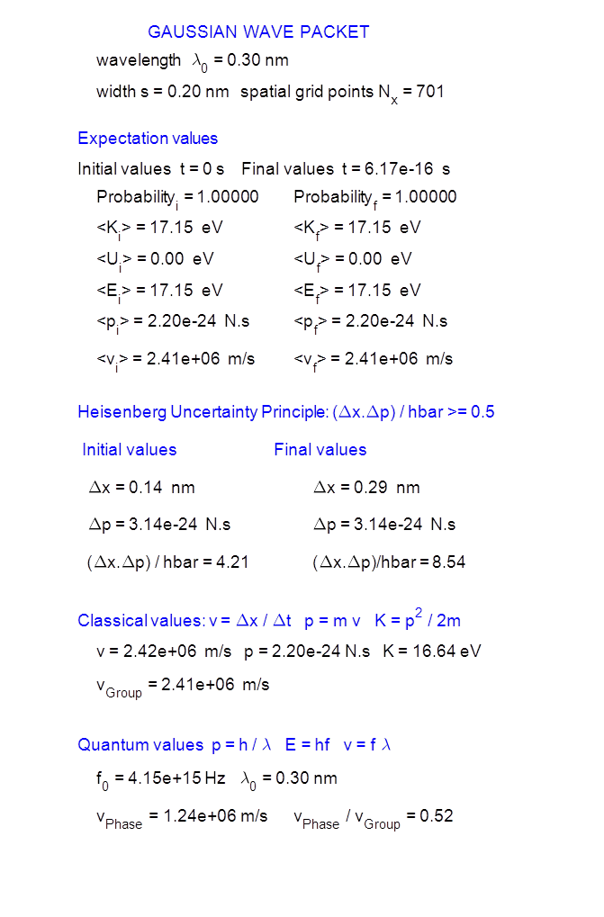
therefore increases the rate at which the wavepacket spreads. Table 1.
Summary of the simulation parameters and computed results. The classical
values are determined by the calculating the velocity
The
wavepacket is a mixture of waves moving at a whole range of velocities, so as
it moves along, some of these components move faster than others. Soon this dispersion causes the wavepacket to spread
out (just as a large group of hikers naturally spreads out along the trail,
with the faster ones in
the lead and the slower ones behind). Although the wavelength of the
oscillations within the packet is initially uniform, it will not remain
uniform. The wavepacket moves and spreads, its leading edge will contain
shorter-wavelength (higher-velocity) oscillations, while its trailing edge
will contain longer-wavelength (lower-velocity) oscillations. Meanwhile the
peak amplitude of the wavepacket will decrease, to conserve probability as
the width increases as illustrates in the animation of figure 1. The
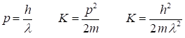
initial kinetic energy K and its momentum p of our electron (mass me) can be estimated from its wavelength Using the default values for the simulations: which are in agreement with the expectation values given in Table 1. All that can happen to a classical particle is
that it can move from one position to another. But, a quantum mechanical
wavepacket undergoes a more complicated evolution with time in which the
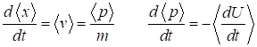
whole probability distribution shifts and spreads with time. The Ehrenfest’s theorem is a general statement about the rates of change
of Ehrenfest’s theorm If a particle of mass m is in a state described by a normalized
wavefunction in a system with a potential energy function In this simulation, you can see that Ehrenfest’s theorem is satisfied. The momentum and
its uncertainty remain constant. The distance d that the peak of the probability distribution
moves in the time interval
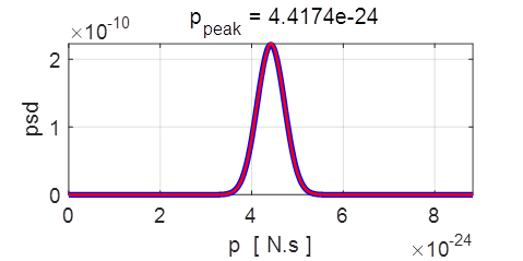
We can
perform a Fourier transform on the wavepacket function to compute the power
spectrum density (psd) in momentum space
Fig.
3. Power spectral density
functions in momentum space ( blue:
t(0), red;
t(end) ). The Fourier transform of a Gaussian function is a Gaussian
function. Top graph ( The Fourier
transform is computed by integration of the Fourier integral and not by the FFT method % Fourier
transform PSI at t = 0 K =
1/wL xMin = 0; xMax = L; KMax =
2/wL0; KMin= -KMax; nK = 2001; K = linspace(KMin,KMax,nK); hP
= psiR(1,:);
HP = zeros(1,nK); for c
= 1:nK g = hP.* exp(1i*2*pi*K(c)*x); HP(c) = simpson1d(g,xMin,xMax); end % HP = HP./max(HP); psd
= conj(HP).*HP; hP = psiR(Nt,:); HP = zeros(1,nK); for c
= 1:nK g = hP.* exp(1i*2*pi*K(c)*x); HP(c) = simpson1d(g,xMin,xMax); end You can also visualize
the complex phase of the wavepacket,
where a colour is used to represent the phase between the real and imaginary
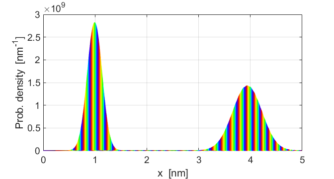
components. Figure 4 shows the complex phase of the Gaussian wavepacket at
the start and end of the simulation period. Figure 5 shows an animation of
the changing complex phase changes as the wavepacket propagates. The Script
runs very slowly when the animation shown in figure 5 is displayed in a
Figure Window.
Fig. 4. The complex phase of the
Gaussian wavepacket at the start and end of the simulation period.
Fig. 5. Animation of the complex phase as
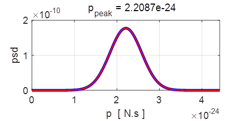
the Gaussian wavepacket propagates. The following
results are the outputs displayed by running the simulation with a doubling
of the nominal wavelength. Since the nominal wavelength is doubled, then the nominal
momentum and group velocity are halved. So, the wavepacket will only travel
half the distance in the same time interval of 0.62 fs.
|