|
MATLAB
RESOURCES QUANTUM
MECHANICS
Ian
Cooper matlabvisualphysics@gmail.com TIME DEPENDENT SCHRODINGER EQUATION FINITE DIFFERENCE TIME DEVELOPMENT METHOD FREE PARTICLE: MOTION OF A WAVEPACKET IN A UNIFORM
ELECTRIC FIELD DOWNLOAD DIRECTORY
FOR MATLAB SCRIPTS simpson1d.m Function for [1D] integration QMG24E.m Propagation of Gaussian wavepacket in a
uniform electric field . LINKS link
[1D] time dependent Schrodinger Equation
using the Finite Difference Time Development Method (FDTD). link Expectation values link
Gaussian wavepacket propagation Motion of an
electron in a uniform electric field We can simulate the motion of a wavepacket representing an electron in
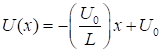
a uniform electric field. The force acting on the electron is derived from
the potential energy function (1) For a uniform electric field, the force acting on the electron is
constant, therefore, the potential energy is a linear function with position x of the form (2) where L is the width of the simulation region and We can solve the time dependent Schrodinger equation using the finite
difference time development method (TDSE/FDTD)
to compute the wavefunction of a Gaussian wavepacket
as a function of time. I
will consider a single electron in the uniform electric field. The electron is represented by a wavepacket
to localize
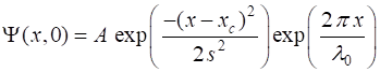
it. An initial state
described by the Gaussian function is
(3) where A is a
normalized constant and is calculated so that Once, the wavefunction is known than the expectation
values of any observable quantities of the wavepacket can be
evaluated:
<x>
position
<p>
momentum
<K> kinetic
energy <U> potential
energy
<E> total
energy The momentum of the wavepacket (the electron) is calculated from the nominal
wavelength
(4) From equations 1 and 2, we can calculate the uniform acceleration a of the wavepacket
(5) The initial values (t = t1 = 0)
are represented by the subscript 1 and final values at time (t = t2). The initial velocity are final
velocities are
The initial and final displacements
are
The initial and final momenta, and
impulse are
The initial and final kinetic
energies, and work done are
The initial and final potential
energies are
The initial and final total energies
are
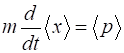
We can apply Ehrenfest’s theorem to
calculate the changes in expectation values, that is, we can apply the
principles of classical physics only to expectation values and not
instantaneous values or not for eigenvalues
Even though we don’t know exactly where the electron is or its exact
velocity at any instant, we can predict with certainty the time evolution of
the probability distribution function and expectation values. Table 1 shows
that there is excellent agreement between the classical predictions and the
numerical results from the solution of the Schrodinger Equation. Table 1. Summary of the simulation parameters and computations.
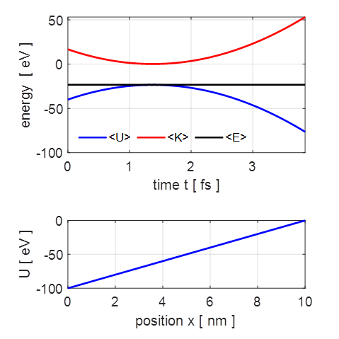
The result summary in Table 1 shows the classical concept of
conservation of energy holds in our quantum system. The total energy of the
system is time independent and any change in the expectation value of the
potential energy is accompanied by a corresponding change in the expectation
value of the kinetic energy. For example, the electric force does work on the
electron to increase its kinetic energy and this is shown by the increase in
the expectation value of the kinetic energy and the decrease in the
expectation value of the potential such that the expectation value of the
total energy does not change (figure 1).
Fig. 1. The time evolution
of the expectation values for the kinetic energy, potential energy
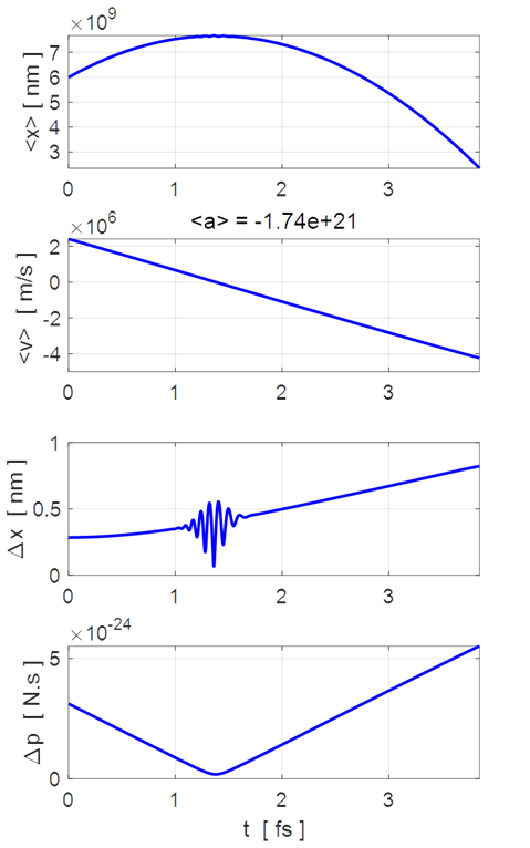
Fig. 2. The time evolution of the expectation values for position and
velocity, and the uncertainties in position and momentum.
Fig. 3. Animation of
the motion of the wavepacket. The wavepacket undergoes wavepacket spreading and with increasing
uncertainties in position and momenta. The wavepacket undergoes a reflection
around x = 8 nm where
the faster components of the wavepacket are travelling to the left while the
slower components are still travelling to the right. The opposite travelling
waves interfere with each other leading to rapid oscillations in both the
real and imaginary parts of the wavefunction. However, the probability
density function remains its Gaussian profile but with an increased width
produced by the reflection. The reflection occurs around t = 1.2 fs and the
interference of the forward and backward waves produces the interesting
changes in the uncertainties in position and momentum (figure 2). The electron can be though as a particle and the
classical laws of physics can be used to predict the time evolution of
expectation values. But the wave nature of the electron means that we do not
know the precise values of position and velocity at an instant. We
can’t predict the path of an electron, we can
only predict the probability of finding the electron at each instant within a
range of x values. Thus, we can conclude that the
expectation value for position tracks the classical trajectory. |