DOING PHYSICS WITH MATLAB IZHIKEVICH MODEL FOR NETWORKS OF COUPLED NEURONS
Matlab Download Directory ns_Izh022.m Computation of the membrane potential activity for a sparse network of randomly coupled neutrons ns_IZH_N012.m [2D] Neural network with Mexican hat coupling function

The Izhikevich model for a neuron can be used to simulate a sparse network of 10³ spiking cortical neurons with 10⁶ synaptic connections. Based upon the anatomy of a mammalian cortex, ratio of excitatory to inhibitory neurons is taken to be 4 to 1 with inhibitory synaptic connections stronger than the excitatory synaptic connections.

Regular spiking cells are used to model all excitatory neurons and fast spiking neurons for the inhibitory neurons.

Also, each neuron receives a noisy thalamic input (presynaptic input into areas of the cerebral cortex from the thalamus). All neurons have different dynamics for heterogeneity. This is done by assigning to each neuron a range of values for the parameters a, b, c and d using the uniformly distributed variables r_e and r_i which vary from 0 to 1.

The time evolution of the membrane potential v is described in terms of the differential equations

(1)

(2)

The after-spike resetting relationship is

(3)

where u is the membrane recovery variable.

The dimensions and values of the model parameters are

v membrane potential [mV]

t time [ms]

dv/dt time rate of change in membrane potential [mV.ms^-1 or V.s^-1]

u recovery variable [mV]

I external current input to cell (synaptic currents or injected DC-currents) [A]

c₁ = 0.04 mV^‑1.ms^-1 c₂ = 5 ms^-1 c₃ = 140 mV.ms^-1 c₄ = 1 ms^-1 c₅ = 1 [mV.ms^-1.A^-1 Ω.ms^-1]

Excitatory cells (variations in c and d)

Regular spiking cells a = 0.02 b = 0.20 c = -65 d = 8

Chattering cells a = 0.02 b = 0.20 c = -50 d = 2

c = - 65 + 15 r_e² d = 8 – 6 r_e²

r_e = 0 corresponds to regular spiking cell

r_e = 1 corresponds to the chattering cell

r_e² used to bias the distribution toward regular spiking cells.

Inhibitory cells (variations in a and b)

Fast Spiking cells a = 0.02 + 0.08 r_i b = 0.25 - 0.05 r_i c = -65 d = 2

Part of the mscript ns_Izh022.m for simulation of mammalian cortex network

% INPUT PARAMETERS ===============================================

Ne = 800; Ni = 200; % number of excitatory & inhibitory neurons

Nt = 1000; % number of time steps

numE = 10; numI = Ne + 10;

% indices for one excitatory and one inhibitory neuron

% Model parameters ===============================================

re = rand(Ne,1); ri = rand(Ni,1); % random numbers

a = [0.02 * ones(Ne,1); 0.02 + 0.08*ri];

b = [0.20 *ones(Ne,1); 0.25 - 0.05*ri];

c = [-65+15*re.^2; -65*ones(Ni,1)];

d = [8-6*re.^2 ; 2*ones(Ni,1)];

S = [0.53*rand(Ne+Ni,Ne), -rand(Ne+Ni,Ni)];

% coupling strengths

v = -65*ones(Ne+Ni,1); % Initial values of v

u = b.*v; % Initial values of u

firings = []; % spike timings

vE = zeros(Nt,1); vI = zeros(Nt,1);

% membrane potential of 2 neurons

% Time Evolution of Systems =======================================

for t = 1:Nt

I = [5*randn(Ne,1);2*randn(Ni,1)]; % thalamic input

fired = find(v>=30); % indices of spikes

firings = [firings; t+0*fired,fired];

% time steps / fired neurons

v(fired) = c(fired); % membrane potential

u(fired) = u(fired)+d(fired); % recovery potential

I = I+sum(S(:,fired),2); % thalamic + synaptic input

v = v+0.5*(0.04*v.^2+5*v+140-u+I); % HALF-STEP: step 0.5 ms

v = v+0.5*(0.04*v.^2+5*v+140-u+I); % for numerical stability

u = u+a.*(b.*v-u);

vE(t) = v(numE); % excitatory neuron

vI(t) = v(numI); % inhibitory neuron

end;

vE(vE > 30) = 30;

vI(vI > 30) = 30;

tS = 1:Nt; nF = zeros(Nt,1); % fired neurons at each time step

for t = 1 : Nt

nF(t) = sum((firings(:,1) == t));

end

The model belongs to the class of pulse-coupled neural networks (PCNN) where the synaptic connection weights between the neurons are given by the matrix S so that firing of the n^th neuron instantaneously changes membrane potential variable v_m by S(m, n).

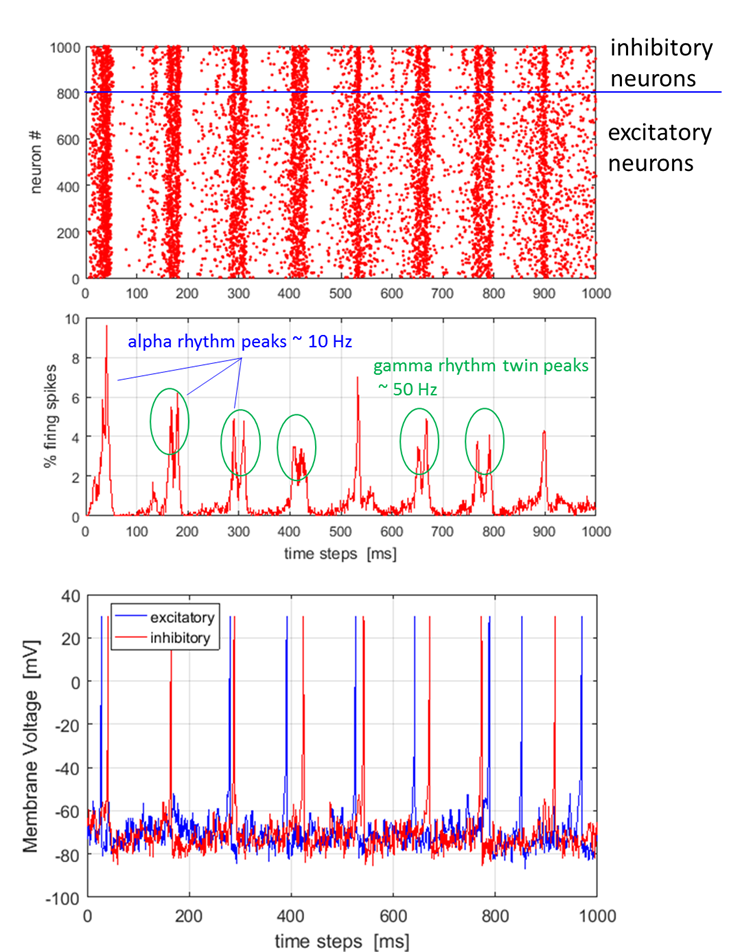
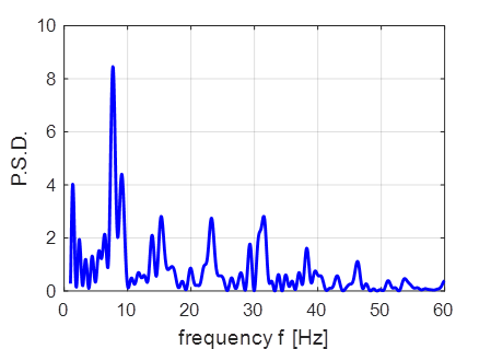
Fig. 1. Network of 10³ randomly coupled spiking neurons (800 excitatory and 200 inhibitory) with 10⁶ synaptic connections. Top: spike-train raster plot shows episodes of alpha rhythms (single widely spaced peaks) and gamma band rhythms (double closely spaced peaks). Bottom: Typical spiking activity of an excitatory neuron and an inhibitory neuron (peaks normalized to +30 mV).

The Foureir transform of the number of firings at each time step is shown in figure 2. Figure 2 shows a distinct each near 8 Hz which may correspond to the episodes of the alpha rhythms. Howver, the Fourier transform does not indicate the gamma rythym oscillations.

Fig. 2. Fourier trnasform of the number of firings at each time step.

Neural activity in the neocortex is highly irregular and the origin of this irregular activity may be in the tight balance between excitatory and inhibitory synaptic inputs. Highly fluctuating net input currents whose means are below threshold results in action potentials being generated by the fluctuations. Neural activity in this state is chaotic in the sense that slight changes in initial conditions leads to drastically different patterns of spike times. The network of neurons in the asynchronous state displays activity that looks random where the firing rate at which action potentials are emitted stochastically. Figure 1 shows that the network exhibits cortical-like asynchronous dynamics (neurons fire Poisson spike trains: excitatory neuron firing rate ~ 7 Hz and inhibitory firing rate ~ 8 Hz). The neurons self-organize into assemblies in which different neurons asynchronously emit action potentials and they exhibit collective rhythmic behaviour in the frequency range corresponding to that of the mammalian cortex in the awake state and although the network is connected randomly and there is no synaptic plasticity.

The alpha rhythm corresponds to the normal bursts of electrical activity within the frequency range from 8 to 13 Hz in the cerebral cortex of a drowsy or inactive person. The gamma rhythm is the burst of electrical activity at higher frequencies than the alpha rhythm within a frequency between 25 and 100 Hz with 40 Hz a typical value. The Izhikevich model may show some evidence of these rhythms. The dark red vertical lines in figure 7 (top diagram) indicate that there are occasional episodes of synchronized firings where single peaks show alpha rhythm (~10 Hz) and double peaks show the gamma rhythm (~50 Hz).

Ostojic concluded from his modelling of sparsely connected network of spiking neurons of excitatory and inhibitory leaky integrate-and-fire (LIF) neurons that they can display two different types of asynchronous activity when at rest:

· For weak overall synaptic couplings and/or strong inhibition, the network is in the well-known asynchronous state, in which individual neurons fire irregularly at rates that are constant in time.

· For overall synaptic couplings that are strong and/or inhibition is just strong enough to balance excitation, a new type of resting state emerges. In that state the neurons still fire irregularly and asynchronously, but the firing rates of individual neurons fluctuate strongly in time and across neurons. This new state is called the heterogeneous asynchronous state.

Ostojic: “The two regimes of spontaneous asynchronous activity have different computational properties, as seen in their responses to temporally varying inputs. In the classical asynchronous state, the responses of different neurons are highly redundant, which favors a reliable transmission of information but limits the capacity of the network to perform nonlinear computations on the stimuli. In the heterogeneous asynchronous state, the responses of different neurons to the input instead strongly vary. This variability in the population degrades the transmission of information but provides a rich substrate for a nonlinear processing of the stimuli, as performed, for instance, in decision-making and categorization.”

Using the mscript nsIzh022.m, you could investigate other types of collective behaviour such as spindle waves ? and sleep oscillations ? by changing the relative strength of synaptic connections and the strength of the thalamic input. Also, you could verify the findings made by Ostojic using the Izhikevich model rather than the leaky integrate-and-fire model.

I am not sure how useful is this model is because the model is sensitive to the model parameters and it is difficult to judge what parameter values to use.

Izhikkevich Quadratic Model:

[2D] NEURAL NETWORK WITH MEXICAN HAT COUPLING FUNCTION

We can simulation the generation of spiking neuron pattern formations called clusters and their propagation characteristics using the Izhikevich Quadratic Model for Spiking Neurons using a [2D] square lattice of N x N uniformly spaced neurons. The time evolution of the membrane potential for each neuron is calculated using a Mexican-Hat function for the coupling between neurons.

ns_IZH_N012.m

Parameters:

% Number of N x N lattice elements

N = 100;

% Number of time steps

NT = 200;

% Izhikevich Model parameters

C = 50; vr = -60; vt = -40; k = 0.7;

a = 0.01; b = 5; c = -55; d = 150;

vPeak = 35;

Sext = 20;

% Coupling Strength function

CE = 0.4;

CI = 0.1;

dE = 14;

dI = 42;

dM = 15;

d0 = 5.4;

WE = 8000;

WI = -8000;

Fig. 4a. Animation of of the time evolution of the membrane potential. contourf plot (left) of membrane potential and plot of spiking neurons (right). ns_IZH_N012.m
Difficult to know what parameters to use. Need extremely large value values for Mexican Hat Function parameters WE and WI. Can get wobbling cluster formations but as yet could not simulate propagating clusters.
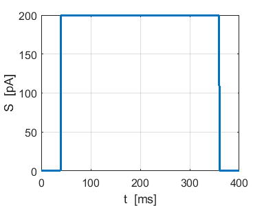
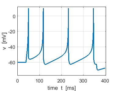
Fig. 4b. Single neuron with the same Izhikevich paramters used for the simulation shown in figure 4a. ns_Izh_006.m